Project for ClimateHack.AI 2023-24 in collaboration with Open Climate Fix.
Accomplishments
- Top 3 Submission from the University of Toronto
- Represented the University of Toronto at the International Finals at Harvard
- Finished 5th place overall, beating out teams such as CMU, Harvard, UIUC, etc
You can view the slides we used for the presentation here: Climate Hack 2023 Final.pdf
Challenge
ClimateHack.AI 2024
Motivation
- Electricity system operators ensure in real time that electricity can always be supplied to meet demand and prevent blackouts, but intermittent renewable energy sources, such as solar and wind, introduce significant uncertainty into the grid’s power generation forecasts.
- To account for this uncertainty, electricity system operators maintain a spinning reserve based on non-renewable energy sources (e.g. natural gas) that can quickly ramp up to meet any shortfalls.
- More accurate near-term solar power generation forecasts would allow grid operators to reduce this use of non-renewables and cut emissions by up to 100 kilotonnes per year in Great Britain and on the order of 50 megatonnes per year worldwide by 2030.
Challenge
- In the 2023-24 competition, Open Climate Fix challenged our participants to develop accurate, efficient machine learning models for predicting solar power generation at the level of individual sites up to four hours ahead.
- Over 600 gigabytes of EUMETSAT satellite imagery, Deutscher Wetterdienst numerical weather predictions, ECMWF air quality forecasts and historical solar power generation data collected from live PV systems in the UK were made available to participants to build their models.
- All in all, 3,900+ models were uploaded by competition participants to the DOXA AI platform for evaluation, and the contributions of the competition will support the solar power nowcasting research of Open Climate Fix.
- Find out more about this year’s challenge on the competition page.
Our Solution
At a high level, our solution had four primary subsystems: a data management layer, a data processing pipeline, a model training pipeline, and a deployment system.
Data Management
Dataset
- We acquired multi-modal datasets from the competition AWS S3 bucket and then stored them locally.
| Data Type | Source Format | Temporal Resolution | Spatial Resolution | Processing Function |
|---|---|---|---|---|
| PV Generation | .parquet | 5 minutes | Site-specific | filter_by_site['pv'] |
| Satellite HRV (high-res) | zarr | 5 minutes | 128x128 pixels | filter_by_site['satellite-hrv'] |
| Satellite Non-HRV | zarr | 5 minutes | 128x128x11 channels | filter_by_site['satellite-nonhrv'] |
| Weather Data | zarr | 1 hour | Variable grid | filter_by_site['weather'] |
| Aerosol Data | zarr | 1 hour | 128x128x8 channels | filter_by_site['aerosols'] |
| From our analysis, the most important data was: |
- PV generation
- Satellite HRV
- Weather:
- Diffusive shortwave radiation (
aswdifd_s) - Direct shortwave radiation (
aswdir_s) - Cloud cover (%)
- High cloud cover (
clch) - Medium cloud cover (
clcm) - Total cloud cover (
clct)
- High cloud cover (
- Relative humidity (%) at 2 meters (
relhum_2m)
- Diffusive shortwave radiation (
- Time:
- Only evaluated between sunrise and sunset
Data organization
The way we spatially indexed our data was via a JSON format like this:
indices.json
{
  "hrv": {"site_id": [x_coord, y_coord]},
  "nonhrv": {"site_id": [x_coord, y_coord]},
  "weather": {"site_id": [x_coord, y_coord]},
  "aerosols": {"site_id": [x_coord, y_coord]}
}
Each site ID maps to an (x,y) pixel coordinate within the respective data grids (allows for extraction of 128x128 pixel windows around each PV site location).
We also made use of the PV site metadata (solar panel orientation, sol panel tilt, peak capacity in kilowatts, installation date) as well as the solar time of each record.
Note that each modality used different spatial resolutions, so we had to also have distinct coordinate systems for the same physical locations. As an example, a site might map to the coordinates [222, 121] in HRV imagery but also map to [119, 133] in non-HRV data.
This indexing was super important because of the following reasons:
- Multimodal alignment; since we had so many different types of data with different spatial/temporal resolutions, we needed a way to properly align them in time and space for the training of a single model.
- Efficient site-specific data retrieval; for example, for satellite data we would extract a 128x128 pixel window centered on the site’s coordinates rather than loading in entire satellite images (way more efficient since we only need small regions around each solar panel site)
Data Processing
The data processing consisted of two main components:
- Feature extraction utilities that handled the temporal + spatial filtering of multimodal data sources
- i.e. creating those spatial/temporal windows for relevant data
- Data loading infrastructure that implemented PyTorch datasets with multi-GPU support
- Time slice creation (generating temporal windows for each feature type)
- Temporal filtering
- Site iteration (processing each PV site sequentially)
- Spatial filtering
- Shape Validation
- Feature assembly
Model Architecture
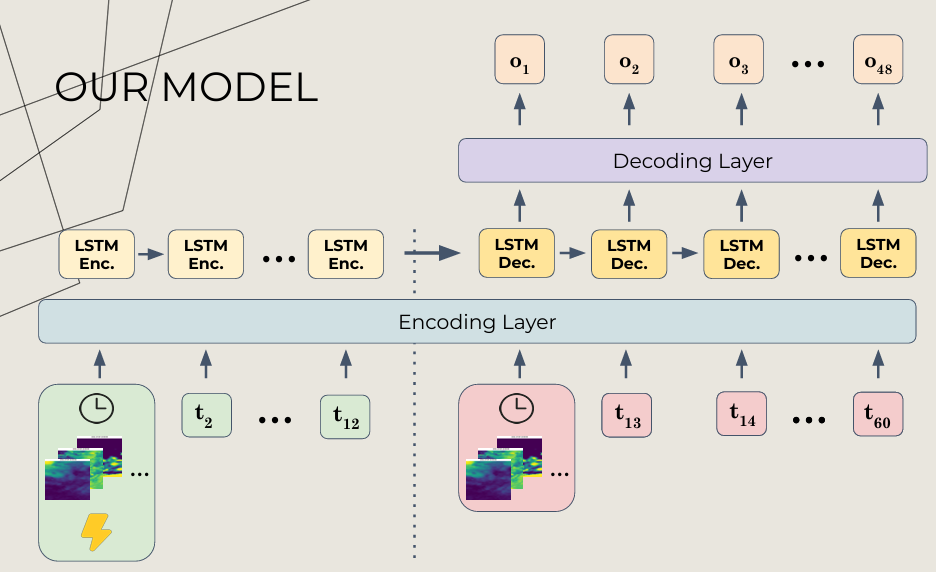
We tried many different model architectures, the best performing one being a seq-to-seq LSTM. For the satellite imagery, it is processed by ConvLSTM cells that handle 2D spatial data. So the inputs are 5D tensors of shape (batch, time, channels, height, width), we run 2D convolutions for all gate operations, and output spatiotemporal feature representations.
class ConvLSTMCell(nn.Module):
    """ConvLSTM Cell"""

    def __init__(
        self,
        input_dim: int,
        hidden_dim: int,
        kernel_size: int,
        bias=True,
        activation=torch.tanh,
        batchnorm=False,
    ):
        """
        ConLSTM Cell

        Args:
            input_dim: Number of input channels
            hidden_dim: Number of hidden channels
            kernel_size: Kernel size
            bias: Whether to add bias
            activation: Activation to use
            batchnorm: Whether to use batch norm
        """
        super(ConvLSTMCell, self).__init__()

        self.input_dim = input_dim
        self.hidden_dim = hidden_dim

        self.kernel_size = kernel_size
        self.padding = kernel_size // 2, kernel_size // 2
        self.bias = bias
        self.activation = activation
        self.batchnorm = batchnorm

        self.conv = nn.Conv2d(
            in_channels=self.input_dim + self.hidden_dim,
            out_channels=4 * self.hidden_dim,
            kernel_size=self.kernel_size,
            padding=self.padding,
            bias=self.bias,
        )

        self.reset_parameters()

    def forward(self, x: torch.Tensor, prev_state: list) -> tuple[torch.Tensor, torch.Tensor]:
        """
        Compute forward pass

        Args:
            x: Input tensor of [Batch, Channel, Height, Width]
            prev_state: Previous hidden state

        Returns:
            The new hidden state and output
        """
        h_prev, c_prev = prev_state

        combined = torch.cat((x, h_prev), dim=1)  # concatenate along channel axis
        combined_conv = self.conv(combined)

        cc_i, cc_f, cc_o, cc_g = torch.split(combined_conv, self.hidden_dim, dim=1)

        i = torch.sigmoid(cc_i)
        f = torch.sigmoid(cc_f)

        g = self.activation(cc_g)
        c_cur = f * c_prev + i * g

        o = torch.sigmoid(cc_o)

        h_cur = o * self.activation(c_cur)

        return h_cur, c_cur
The weather data is encoded via a linear embedding
self.weather_emb = nn.Sequential(
    norm_layer,                    # Batch or global normalization
    nn.Flatten(start_dim=2),       # Flatten spatial dimensions
    nn.Linear((len(weather_features)) * WEATHER_SIZE ** 2, weather_emb_dim)
)
The primary LSTM encoder combines all embedded features:
 def start_input_state(self, features, index):

        batch_size = features[0].shape[0]

        inp_t = torch.arange(12, device=features[0].device, dtype=torch.int32)[None].repeat(batch_size, 1) # B 12
        inp_emb = torch.cat([features[0].unsqueeze(-1), features[1][torch.arange(batch_size)[:, None], (index + inp_t) // 12]], axis=-1)
        if self.kwargs['use_time']:
            inp_emb = torch.cat([inp_emb, features[2].repeat(1, 12, 1)], axis=-1)
        if self.kwargs['use_site']:
            inp_emb = torch.cat([inp_emb, features[3].repeat(1, 12, 1)], axis=-1)
        inp_emb = torch.cat([inp_emb, self.pos_emb(inp_t)], axis=-1)
        return inp_emb
class BaseLSTM(nn.Module):
def __init__(self, enc_model, dec_model, inp_emb, dropout=0.2, **kwargs):
self.enc_model = enc_model
self.dec_model = dec_model
self.inp_emb = inp_emb
self.used = [kwargs.get(f'use_{k.replace("-", "_")}', True) for k in ['pv', 'satellite-hrv', 'satellite-nonhrv', 'aerosols', 'weather', 'time', 'site']]
self.dropout = nn.Dropout(p=dropout)
def emb_input(self, features):
pv, *features, index = features
return (pv, *[emb(feat) for feat, emb in zip(features, self.inp_emb)], index)
def forward(self, features, target, criterion):
*features_emb, index = self.emb_input(features)
_, tup = self.enc_model(self.dropout(self.start_input_state(features_emb, index)))
last_out = F.pad(features[0][:, -1, None], (0, self.dec_model.proj_size - 1), 'constant', 0)
loss = 0
for i in range(48):
out, tup = self.dec_model(self.dropout(self.next_input_state(i, last_out, features_emb, index, target)), tup)
out = self.output_state(i, out, last_out)
loss += criterion(out.squeeze(-1), target[:, i].squeeze(-1))
last_out = out
return loss / 48Model Deployment/Submission
- For submission and evaluation, we use a
Base_EvaluatorClass with asetup()method to load the trained model checkpoint and relevant config files, thepredict()method processes the test data in batches and yields predictions as numpy arrays of shape(batch_size, 48), representing the future 48 timesteps. Finally, theevaluate()method saves these predictions and sends them to the competition platform.
class Evaluator(BaseEvaluator):
    def setup(self) -> None:
        """Sets up anything required for evaluation, e.g. loading a model."""

        self.weather_features = 'aswdir_s aswdifd_s clct relhum_2m'.split()
        self.model = Model(hidden_dim=2048, use_time = True, model_diff=True, use_weather=True, weather_features=self.weather_features, norm_type='global').to(device)
        self.model.load_state_dict(torch.load("checkpoints/last15.pt", map_location=device))
        self.model.eval()

        self.site_cache = json.load(open('site_cache.json'))

    def predict(self, features: h5py.File):
        """Makes solar PV predictions for a test set

        Args:
            features (h5py.File): Solar PV, satellite imagery, weather forecast and air quality forecast features.

        Yields:
            Generator[np.ndarray, Any, None]: A batch of predictions.
        """

        with torch.inference_mode():
            # Select the variables you wish to use here!
            for pv, time, *weather_features in self.batch(features, variables=["pv", "time"] + self.weather_features, batch_size=128):

                weather = np.stack(weather_features, axis=2)[..., 63:65, 63:65]
                arr = dt2cal(time.view('datetime64[ns]'))
                time_one_hot = np.zeros((pv.shape[0], 12 + 31 + 12), dtype=np.float32)
                time_one_hot[np.arange(pv.shape[0])[:, None], arr + np.cumsum(np.array([0, 12, 31]))] = 1.

                predictions = self.model.predict(
                    (torch.from_numpy(pv).to(device),
                    # torch.from_numpy(hrv).to(device),
                    torch.from_numpy(weather).to(device),
                    # torch.from_numpy(arr[:, :-1]).to(device),
                    torch.from_numpy(time_one_hot).to(device),
                    torch.from_numpy(arr[:, [-1]].astype(np.int32)).to(device),
                    )
                ).cpu().detach().numpy()

                ######## SMOOTHING ###########

                full = np.concatenate([pv, predictions], axis=-1) #32 60
                base = 0.70
                N = 8
                wma = base**np.arange(N)
                wma /= wma.sum()

                predictions = np.stack([np.convolve(full_batch, wma, 'valid') for full_batch in full], axis=0)[:, 12 - N + 1:]
                predictions[pv[:, -9:].max(axis=-1) < 0.01] = 0.

                predictions = np.clip(predictions, 0, 1)
                yield predictions